Symmetric and Asymmetric Fermi Surfaces in Kspace

Valentin Urena Baltazar

Hi all! Welcome to my first post for our Physics 156: Solid State class!

IMPORTANT NOTE: Read this Introduction on the Blog and THEN click the links to Parts 1 & 2 at the bottom! They have all the really cool Kspace diagrams I plotted using Python! I also ask some questions there that you all can try and comment on here. Thanks!

First let us begin with  a little introduction to the related subject on this post.

We have been studying energy bands and their related electron states. We tackled 1 Dimension for which the \(E_F(Fermi)\) level is depicted below as two points that bound the electron states below them. For this 1D case we have E(k) as a function of just kx.

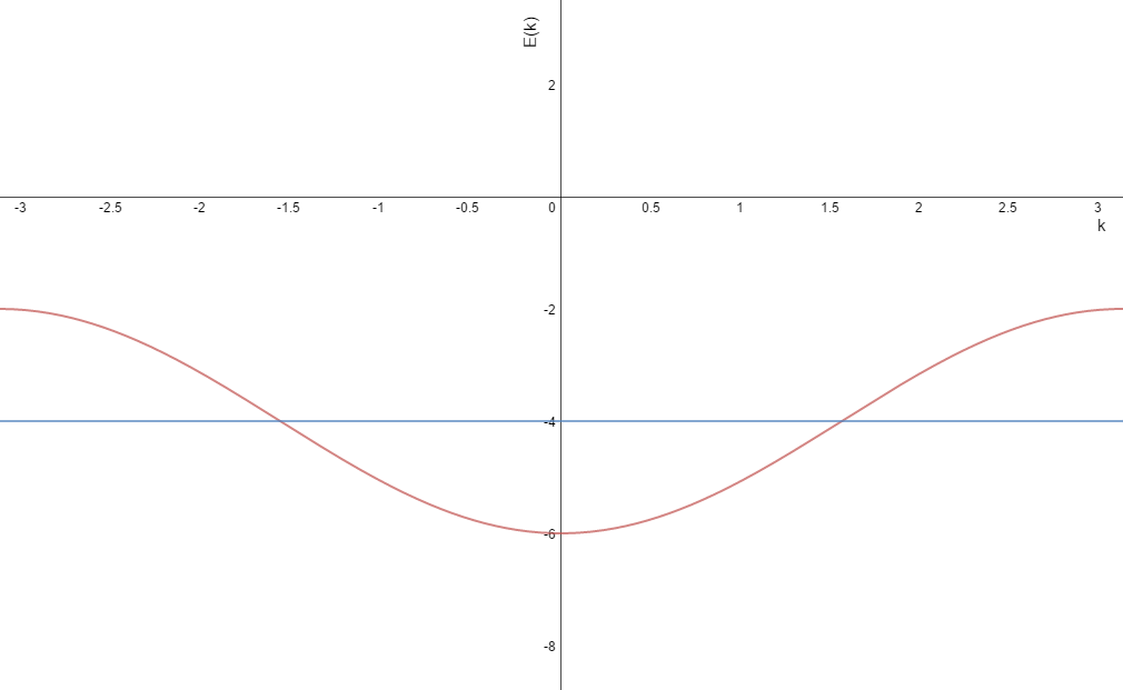Efermi as the blue line

Now we have moved onto 2D models, that is now the \(E_F\) boundary is a line or lines in our \((k_x,k_y)\)space. These “Fermi surfaces” also relate to the energy in that the area within the contours is directly proportional to the fraction of electron states occupied. Everywhere along the contour the energy is constant and the electrons occupy states below that energy which in our \(Kspace\) plot would be the area within the bounds of the contour lines. The total area is always a square of side length \(2\pi /a\) but depending on the \(E_F\) level the area formed within the contours will be some fraction of the total area.

Let us begin with the simplest example: when we have half the total states filled as shown below.

(note: kx is along the X axis and ky along the Y axis for all 2D graphs posted)

The graph above shows the equation \(E(k)=E_0-bcos(ak_x)-bcos(ak_y)\) for the case where \(0=-bcos(ak_x)-bcos(ak_y)\) that is \(E(k)=E_0\). Which we know is the halfway point of our band which ranges from \((E_0-2b,E_0+2b)\)

We will use \(a=.157nm\), \(b=2eV\) and let \(E_0\) just be some constant.

Now the area shown above can be found 2 ways.

1. Geometry! It looks like 4 right triangles of base/height =20. Easy, Area inside the contour = 800. Total area of our \(Kspace\) \((-\pi /a,\pi/a)\) = 1600. Now the fraction of area inside our contour is = 800/1600 = 0.5. So we have HALF the area inside our countor and half outside, this is the expected result for when half our states lie below \(E_F\) (This is true because \(E(k)=E_0\) which is the midpoint).
2. We can rewrite our equation \(-bcos(ak_x)-bcos(ak_y)=C\) as a function \(K_y(k_x)\) such that \(K_y(k_x)=(1/a)\arccos (-C/b-cos(ak_x))\) This will give us the top half of our diagram (otherwise it will not be a proper function) shown below. 
   

   

   Now we integrate from \((-\pi /a,\pi/a)\) and we get a value of 400. Half the value from our geometric approach as expected. Now because of the symmetry of \(Kspace\) we can simply find how many states are filled by finding the ratio of the area above \(k_y=0\) to that of area above \(k_y=0\) but inside our triangle. That is 400/800 = 0.5, same as our geometric approach above! (Note: I have set the equation equal to some value C so that we can range it from \((-2b,2b)\)  thus our \(E(k)\) range now becomes \(E(C)=E_0+C\) (I will explain the usefulness of this later on).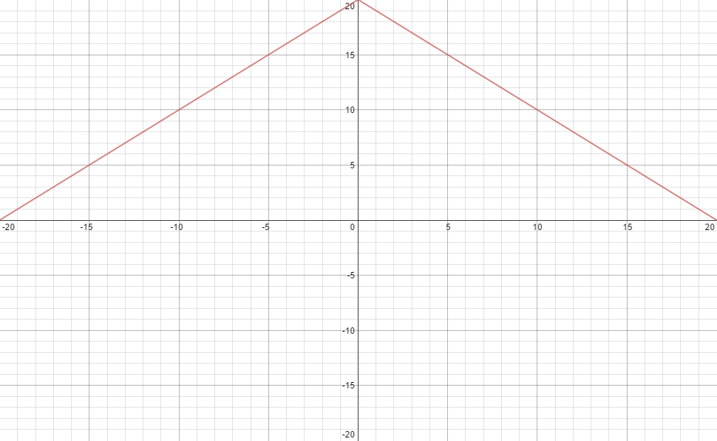

So we can do this method for other values of \(C\) right?...

Well let us look at \(C<0\). The diagram below is for \(C=-3\) using our function \(K_y(k_x)\). 

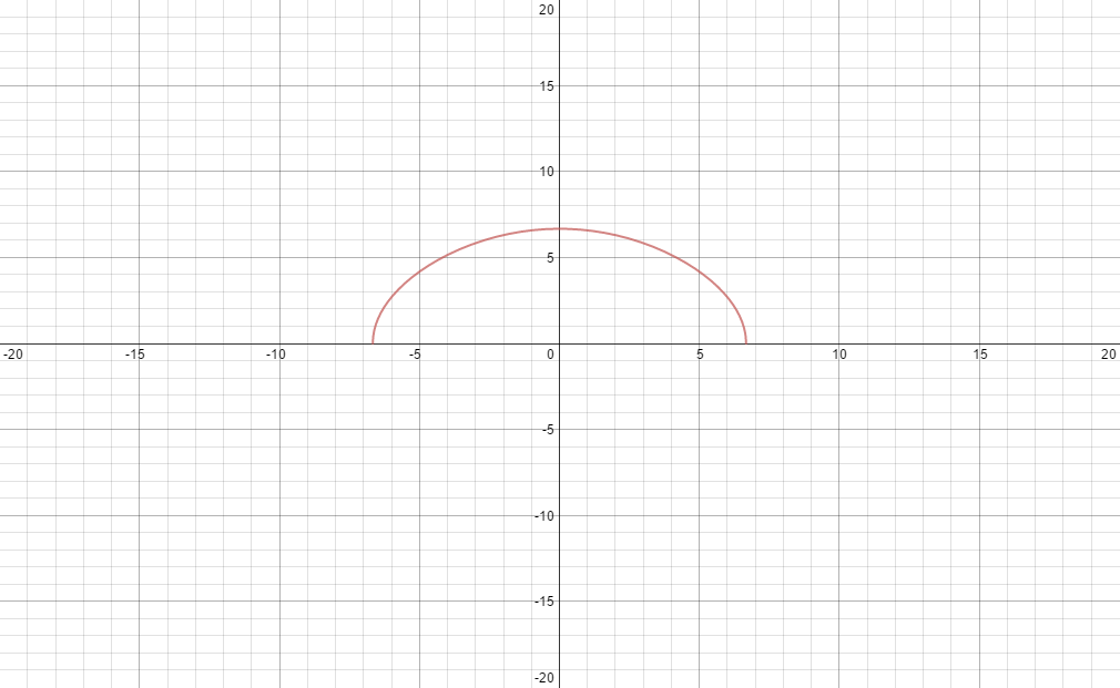
To find the total area geometrically may not be too hard, we can find the bounds and then find the area of the half circle. I am not sure this geometric approximation will be that useful anymore since our shape now is more like an ellipse.

Fear not! Method 2 will work. This is a function bounded on the left and right so let us just integrate (equation) from (-6.67,6.67) and we get about = 68.18. Dividing this by the area above \(k_y=0\)  and we find that about 8.5% of the total area is within our contour. In other words 8.5% of total electron states lie below this \(E_F\) level. (Not surprising since we have set \(C=-3\) which lies near the bottom of our band that ranges from \((E_0-2b,E_0+2b)\) remember \(b=2eV\)).

Ok we are done, we can just use the integral method for all \(C\) ....hmmm not so fast.

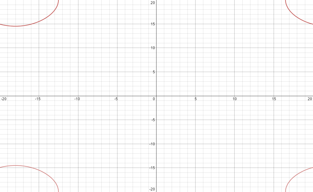
Let us look at \(C>0\), for example \(C=3\) shown below.

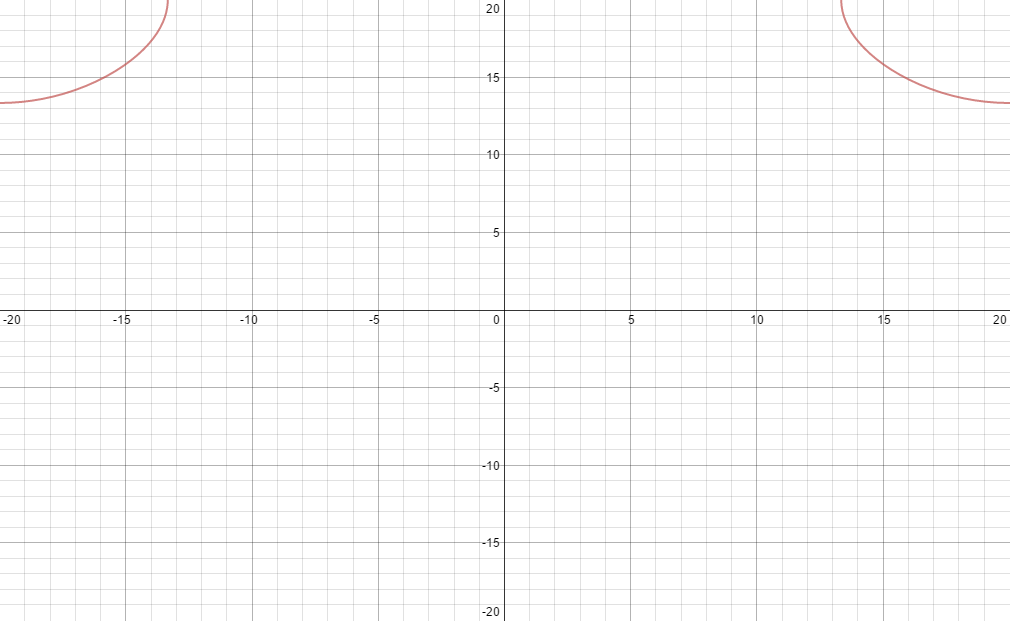
This is a discontinuous function! And our integration method fails as depicted in the picture above. BUT we can find the bounds of one contour (may or may not be too hard) and find the area underneath it and multiply by 2 since we have the same contour on the opposite side. Then use our geometric approach and add the “missing” area between the contours which is in this case a rectangle. This should work but it is a long process.

What about for a case where we have an applied voltage and our \(Kspace\) area is skewed to the +kx direction? As you can see below we still have a piece-wise function but now the contour on the left and right have to have different limits of integration and the areas are no longer have the same area underneath either.

This makes me sad :( 

Sure we can still just find the limits for the left and right side then sum two separate integral and add the missing area inside….but there's an easier way! One which will let us integrate ANY value of \(C\) symmetric or not.

Using Python and a method of integration called the “Monte Carlo” method of integration (and countless hours of coding) I have below links where I show \(Kspace\) diagrams for symmetric and asymmetric cases.

Follow Part 1 then go on to Part 2 to to finish this blog post! Thanks all.

Part 1: Symmetric Kspaces using Monte Carlo Integration

Part 2: Asymmetric Kspaces using Monte Carlo Integration